Positron is finally came out of beta recently, but I notice their download page is showing examples of python visualisation with matplotlib rather than ggplot2. This makes me wondering if the company Posit, previously known as RStudio, had change their ideology in data science.
I had no interests in starting a debate about R vs Python. Personally, I’ve written plenty python code but mainly for bioinformatics intermediate file processing,tool development, workflow and automation. When it comes to data wrangling and visualisation, I’ve done most of my work in R, specicially with the tidyverse for paper publications. I really appreciate the elegance of the grammar of graphics, the simplicity of the pipe operator |>, and the natural way ggplot lets you map variables directly from data frames.
By contrast, I never really studied the matplotlib in depth, and my lasting impression was that the syntax for handling figures and axes felt confusing. Today, I gave it another try. This time, I tried to approach it with a more flexible mindset, treating it as a different philosophy of visualization. Working through some examples made me rethink the way I approach plotting, especially because matplotlib encourages you to engage with its explicit object-oriented interface.
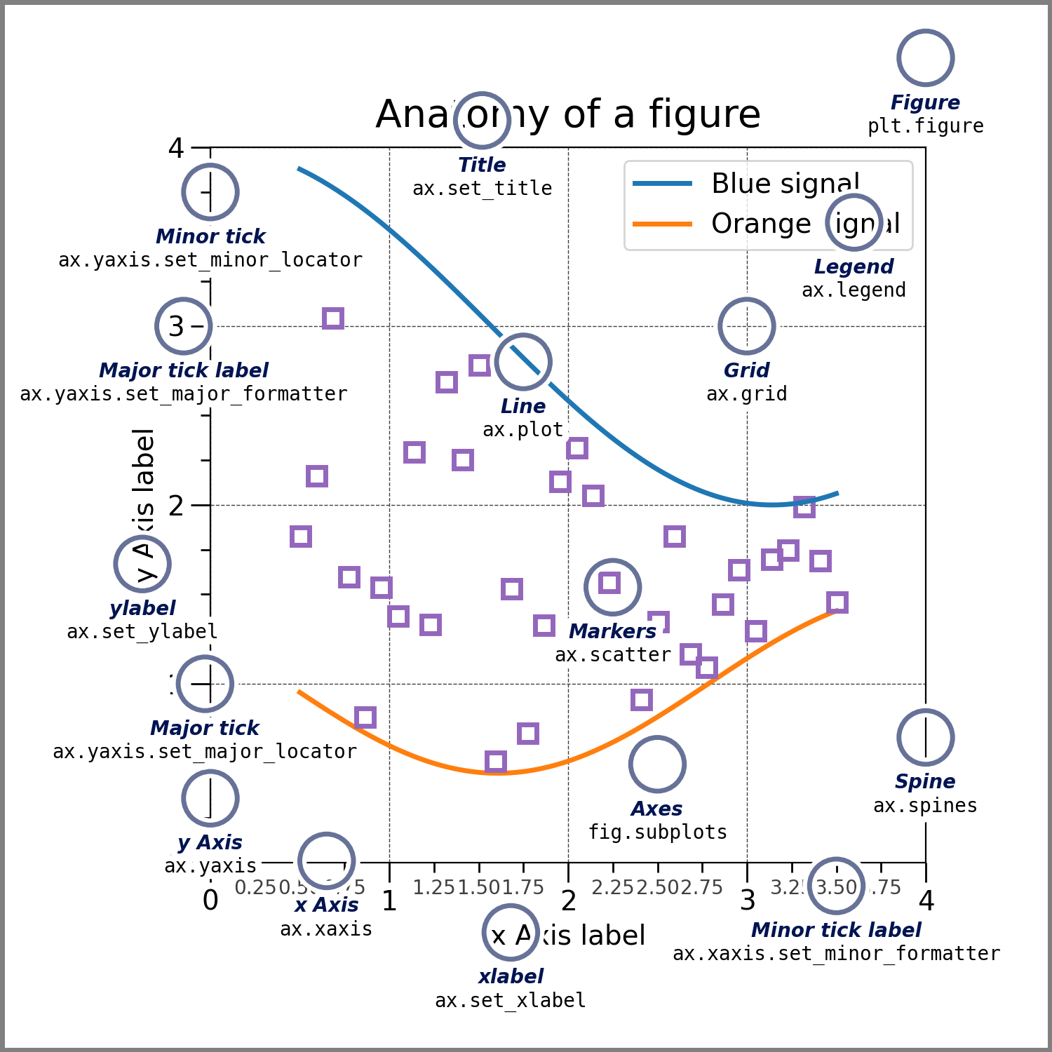
 Components of a matplotlib figure
In matplotlib, you work at the level of objects. A Figure is the entire canvas, and within it, Axes represent individual plotting areas (confusingly named at first). Each Axes contains all the visual elements of a plot.
Mental Model Transitions
When moving from ggplot2 to matplotlib, I really need to restructure mine thinking:
From layers to objects: Instead of adding layers with +, you’re creating objects and calling methods:
# geom_point(aes(x = x, y = y))
fig, ax = plt.subplots()
scatter = ax.scatter(x, y)
ax.set_xlabel('X Label')
From automatic legends to manual construction: Legends in ggplot2 are automatic whereas in matplotlib, you build them yourself
# aes(color = variable)
for category in categories:
    mask = data['category'] == category
    ax.scatter(data[mask]['x'], data[mask]['y'],
              label=category, alpha=0.7)
ax.legend()
From faceting to subplots:
# facet_wrap(~category, ncol = 3)
fig, axes = plt.subplots(2, 3, figsize=(15, 10))
for i, category in enumerate(categories):
    mask = data['category'] == category
    row, col = divmod(i, 3)
    ax.scatter(data[mask]['x'], data[mask]['y'],
              label=category, alpha=0.7)
Adding fitting lines:
# geom_smooth(aes(x = x, y = y), method = 'lm')

from scipy.stats import linregress
slope, intercept, r_value, p_value, std_err = linregress(x, y)
line = slope * x + intercept

ax.scatter(x, y)
ax.plot(x, line, color='red', label=f'R² = {r_value**2:.3f}')
Color palettes: In ggplot2, palettes are built-in. In matplotlib, you manually manage them (or use rcParams)
# scale_color_brewer(palette = 'Set1')

colors = ['#1f77b4', '#ff7f0e', '#2ca02c', '#d62728',
          '#9467bd', '#8c564b', '#e377c2', '#7f7f7f',
          '#bcbd22', '#17becf']
## or using matplotlib.rcParams['axes.prop_cycle'] = cycler.cycler('color', colors)
for i, category in enumerate(categories):
    mask = data['category'] == category
    ax.scatter(data[mask]['x'], data[mask]['y'],
              label=category, alpha=0.7, color=colors[i])
The code to make a similar plot with matplotlib is significantly longer than ggplot2, but the code is actually more readable. I think I will stick with ggplot2 for static visualisation for publications, with the help of gg family of packages, I think ggplot is excellent for generate high-quality figures without extra work. At the same time, I will keep learning matplotlib,not only because of its flexibility, but also because working with its object-oriented structure deepens my understanding of how graphics are built. In many respects, matplotlib feels conceptually closer to D3.js, offering explicit control over higher-level objects and a more fundamental perspective on visualization design.
Another happy thing is that the code train is back:)